Two weeks after results are declared, many colleges circulate a result analysis: pass percentages by programme, by subject, often by section and teacher, sorted from best to worst. Heads of department are asked to explain the bottom of the list. Sometimes those explanations go into appraisals. The table is presented as a measurement, and for a section of 200 students it nearly is. For a section of twelve it is mostly a coin toss with a decimal point.
None of this is new to statisticians. Wainer called the square-root law of sampling variation the most dangerous equation precisely because it keeps producing league tables in which the smallest units crowd the top and bottom. Goldstein and Spiegelhalter showed a quarter of a century ago that institutional rankings need intervals around ranks, not just around rates. Kane and Staiger showed that school accountability systems built on small cohorts reward and punish noise. What has been missing in Indian higher education, as far as we can tell, is a worked comparison on data shaped like ours, with an estimator a college can actually run, and a plain statement of what the table can and cannot say.
Why the extremes are always small
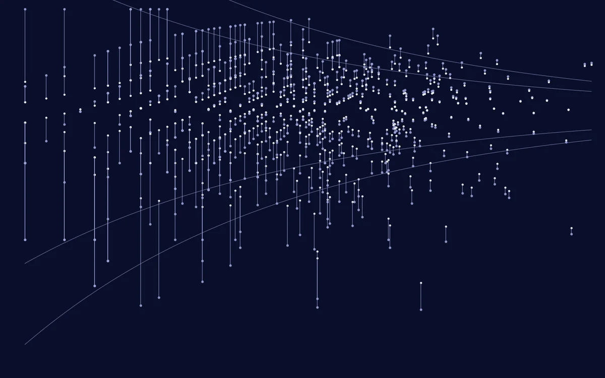
A section of n students with a true pass rate p produces an observed rate with standard deviation √(p(1−p)/n). At p = 0.78 that is 13 points for a section of ten and 2.9 points for a section of two hundred. When the true rates themselves vary by only a few points between sections, as they do, sampling noise dominates the spread of the small sections and they occupy the tails of any sorted table.
Spiegelhalter’s funnel plot, above, is the right first picture and we recommend that every college publish one instead of a sorted list. But a funnel answers only ‘is this section unusual given its size’. It does not give a better estimate of the section’s rate, and it does not say how confident we should be in its rank. For that we need a model of how true rates vary.
Three estimators
All three treat each section’s true rate as a draw from a distribution and combine the section’s own data with that distribution in proportion to how informative the data are. They differ in what the distribution is allowed to depend on.
Beta-binomial empirical Bayes
The simplest: every section’s rate is drawn from a single beta distribution, whose parameters are estimated by maximising the beta-binomial marginal likelihood across all sections. The posterior mean has a closed form:
It shrinks every section toward the college-wide mean by an amount that falls with enrolment, as if each section had borrowed a + b students from the average. Its weakness is that it shrinks a first-year evening section toward the same mean as a third-year laboratory course, which is wrong if those groups genuinely differ.
Fay-Herriot on empirical logits
The small-area estimation workhorse. Transform each section’s rate to an empirical logit with a known sampling variance, and model the true logits as a linear function of section covariates plus a random effect:
With β and τ2 estimated by maximum likelihood, the estimate for each section is a weighted average of its own logit and the regression prediction:
The shrinkage factor Bk is the whole idea in one expression: a section with high sampling variance relative to the genuine between-section variance is pulled hard toward what its characteristics predict.
Binomial logit-normal by marginal maximum likelihood
Fay-Herriot’s normal approximation to the sampling distribution is poor for very small sections and for rates near 100%, both common in result analyses. The exact model keeps the binomial likelihood and integrates over the random effect numerically, here with 40-point Gauss-Hermite quadrature:
Given the fitted hyperparameters, each section’s posterior over its true logit is computed on a grid, which gives the posterior mean rate and, by joint simulation across sections, a posterior distribution for its rank. This is empirical Bayes rather than full Bayes: the hyperparameter uncertainty is ignored, which narrows intervals slightly. With 640 sections the omission is small, and the model runs in under a second.
The simulated college
Result 1: shrinkage is more accurate, by a lot
| Estimator | RMSE (pts) | Rank corr. with truth | Bottom-decile precision | Flags from sections under 25 | Year-to-year rank corr. |
|---|---|---|---|---|---|
| Raw pass percentage | 7.27 | 0.820 | 65.7% | 33.9% | 0.584 |
| Beta-binomial EB | 5.67 | 0.836 | 67.5% | 18.9% | 0.623 |
| Fay-Herriot, covariates | 5.49 | 0.855 | 69.1% | 21.2% | 0.758 |
| Logit-normal MML, covariates | 5.28 | 0.861 | 69.2% | 21.3% | 0.730 |
Every shrinkage estimator beats the raw rate on every metric. The logit-normal model cuts mean squared error by 47%, from a root-mean-square error of 7.3 points to 5.3. The gain is concentrated where it is needed. In a supplementary run of 60 replicates, the raw rate’s RMSE was 10.9 points for sections under 25 students, 6.0 for sections of 25 to 99 and 3.3 for sections of 100 or more; the logit-normal estimate brought those to 6.9, 4.9 and 3.1. Large sections barely move, as they should.
The covariates matter. The beta-binomial model, which shrinks everything toward one college-wide mean, gives most of the accuracy gain but less of the ranking gain, because it pulls genuinely strong third-year laboratory sections and genuinely weaker first-year evening sections toward the same point. Adding course level, mode and type lets the estimator shrink each section toward a sensible comparison group.
Result 2: the small sections leave the tails
Sorted by raw pass percentage, 37% of the sections in the top and bottom deciles come from the smallest quarter by enrolment, half as many again as chance. After shrinkage the share falls to 19%, slightly below a quarter, because a small section now needs a genuinely unusual result, not merely an unlucky one, to reach the extremes. Teachers of small elective and evening sections, who are disproportionately junior and on contract, stop being the people asked to explain the bottom of the list every term.
Result 3: the published table stops lurching
Because the true quality of a section persists (correlation 0.80 between years in the simulation) while sampling noise does not, a good estimator should produce a table that is stable from one year to the next for the right reasons. The raw table’s year-to-year rank correlation is 0.58. The Fay-Herriot table reaches 0.76 and the logit-normal table 0.73. The difference between those two is the one place the cruder model wins: its normal approximation shrinks very small sections slightly harder, which costs a little accuracy and buys a little stability. Either is a large improvement on a table whose year-to-year rank correlation is barely more than half, most of the movement in it being noise.
Result 4: ranks are much less certain than they look
The posterior from the logit-normal model lets us ask the question a principal actually cares about: how sure are we that this section belongs where the table puts it? We draw jointly from every section’s posterior, rank each draw, and report the 5th and 95th percentiles of each section’s percentile rank.
The median section’s 90% rank interval spans 45 percentile points. For sections in the smallest quarter it spans 62; for the largest quarter, 31. A section of ten students with a 60% pass rate, which would sit near the bottom of a raw table, has a 90% interval running from the 5th to the 67th percentile. A section of 215 with a 45% pass rate is, with near certainty, in the bottom 3%. The raw table presents those two facts as the same kind of fact. They are not.
Even among sections in the raw bottom decile, the average posterior probability of truly being in the bottom decile is 66%. One flagged section in three is there by bad luck, and the table gives no way of telling which.
If a college must publish a ranking, it should publish shrunken estimates with rank intervals, and it should not attach consequences to any section whose interval crosses the threshold that triggers them.
What we recommend
- A funnel plot instead of a sorted list, with control limits drawn around the expected rate for the section’s course level and mode.
- Shrunken estimates in every table, for example using the logit-normal model with course level, mode and course type as covariates, fitted per examination session. The raw rate stays visible beside it, because a head of department is entitled to see the number their students actually produced.
- Rank intervals, and a flag rule based on posterior probability rather than position: a section is flagged for review only if the probability that its true rate is below the college’s threshold exceeds 0.8.
- No teacher-level league tables. A teacher’s sections are few, small and assigned non-randomly, which compounds every problem above with selection. Teacher-level funnel plots are defensible for a teacher’s own use and for nothing more.
Method
Limitations
Section quality in the simulation is a stable property plus noise. In reality some of the between-section variation is caused by the students, not the teaching: sections differ in who enrols in them, and shrinkage toward a covariate prediction does nothing about selection unless the covariates capture it. The covariates used here describe the course, not the students; adding entry characteristics would change what the estimate means, from ‘how did this section do’ toward ‘how did it do given who was in it’, which is a value-added question with its own well-documented problems. Pass rates are also bounded and sometimes manipulated by moderation, which a binomial model does not represent. Finally, the empirical Bayes intervals ignore uncertainty in the hyperparameters; a fully Bayesian fit would widen them a little, which only strengthens the argument.
Simulated data only. The estimators, the simulation and the rank-interval code are published. A college that wants to apply them to its own result analysis can do so without sending us any data. Write to team@eduplatter.com.
Related work
Shrinkage begins with Robbins [1] and with Efron and Morris’s demonstration that Stein’s estimator beats raw averages in practice [2]. The empirical-logit model is Fay and Herriot’s [3], and Rao and Molina [4] is the standard reference for small-area estimation. Goldstein and Spiegelhalter [5] set out the case for rank intervals in institutional league tables, and Spiegelhalter’s funnel plot [6] is the display we recommend. Wainer [7] explains why the extremes are always small, and Kane and Staiger [8] document the consequences in school accountability. The logit-normal model and its grid posterior follow standard hierarchical modelling practice [9]. Our earlier efficacy work [10] is the reason we care about precision at small n: programme effects are estimated on exactly these sections.
Artefacts
Everything below is published or available on request. A number nobody can reproduce is an advertisement, not a result. Real institutional records are never shareable under our processor obligations, so where that applies we release a simulated corpus that reproduces the qualitative finding.
References
- Robbins, H. (1956). An Empirical Bayes Approach to Statistics. Proceedings of the Third Berkeley Symposium on Mathematical Statistics and Probability, 1, 157–163.
- Efron, B., & Morris, C. (1975). Data Analysis Using Stein’s Estimator and Its Generalizations. Journal of the American Statistical Association, 70(350), 311–319.
- Fay, R. E., & Herriot, R. A. (1979). Estimates of Income for Small Places: An Application of James-Stein Procedures to Census Data. Journal of the American Statistical Association, 74(366), 269–277.
- Rao, J. N. K., & Molina, I. (2015). Small Area Estimation (2nd ed.). Wiley.
- Goldstein, H., & Spiegelhalter, D. J. (1996). League Tables and Their Limitations: Statistical Issues in Comparisons of Institutional Performance. Journal of the Royal Statistical Society, Series A, 159(3), 385–443.
- Spiegelhalter, D. J. (2005). Funnel Plots for Comparing Institutional Performance. Statistics in Medicine, 24(8), 1185–1202.
- Wainer, H. (2007). The Most Dangerous Equation. American Scientist, 95(3), 249–256.
- Kane, T. J., & Staiger, D. O. (2002). The Promise and Pitfalls of Using Imprecise School Accountability Measures. Journal of Economic Perspectives, 16(4), 91–114.
- Gelman, A., Carlin, J. B., Stern, H. S., Dunson, D. B., Vehtari, A., & Rubin, D. B. (2013). Bayesian Data Analysis (3rd ed.). CRC Press.
- Bhardwaj, M. (2021). Doubly robust estimates of programme effects when uptake clusters by college. EduPlatter Research, EPR-2021-01.
Bhardwaj, M. (2022). Small sections, loud numbers: empirical Bayes shrinkage for course-level result analysis. EduPlatter Research, EPR-2022-01.